Excel is a vast universe of tools that are all designed to store, organize, and (most importantly) manipulate data. For anyone who’s used the program, it’s pretty apparent from the start that even a user working in it for a few years probably only scratches the surface of its power. But you don’t have to be an Excel genius or devote hours to learning complex formulas to start getting more sophisticated benefits out of the application. Scanning through some of the precursory tips can help you advance those you already know. Even refreshing yourself on the basics can get you results since we often gravitate to the few functions we already know and use repeatedly, forgetting those that we don’t practice as much.
We hope this ‘tips & tricks’ article helps you do more with what you already have. And of course, if there’s anything we do to help you with your business applications and their supporting systems, just contact us at Biz@HDCav.com or 360-930-6990.
Tips, Tricks, & Shortcuts
Customize your toolbar with frequent actions
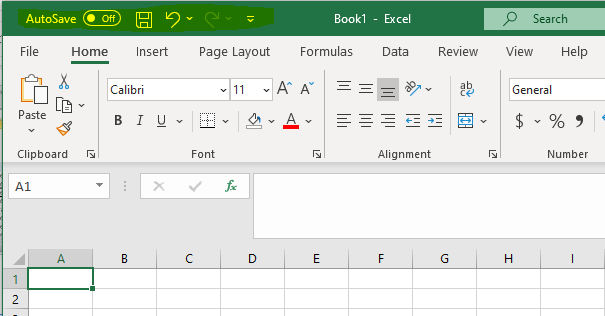
Since there are so many tools to choose from, Excel can sometimes be painstaking to use. Especially when you’re doing repetitive tasks and you want to minimize clicks. That’s why Microsoft provides the Quick Access Toolbar. It just takes a little consideration and time to set it up to save you a lot of both.
In any area or tools you see in the Toolbar, just right click on it and then choose ‘Add to Quick Access Toolbar.’ Then you’ll see that tool appear in the top left near the ‘Save’ icon. To organize them, right click on the area and select ‘Customize Quick Access Toolbar’ which will allow you add, remove, and put them in any order you like.
Select all cells with one click
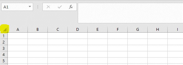
Need to select the whole sheet? Just grabbing the cells you want by clicking and dragging won’t do this, but you can get them all by just clicking on the square where rows and columns meet in the upper left of the data area and you have them all!
Copy/paste only the data you want
Tons of hidden data and formatting can exist in a cell, and you may only want to copy some of it. You can do this using the ‘Paste Special’ functions.
Copy your data by highlighting it and using Ctrl + C or right clicking and selecting ‘Copy.’ Then highlight your destination for the copied data and right click it. Under ‘Paste Options,’ you’ll see a variety of choices, some of the most popular are:
- Values – This option leaves all formatting unchanged so it will only paste the text you see in the cells.
- Formulas – This allow you to keep the formula but the not the formatting.
- Formats – This option allows you to duplicate formats while leaving existing values and formulas.
- Column Widths – this option allows you to paste the data in uniform column widths instead of doing it manually after the paste.
Copy or move a worksheet from one workbook to another
Worksheets can contain a hefty amount of data, formulas, and formatting which can be a nightmare to try to accurately move to manually move. A few simple steps makes this a breeze.
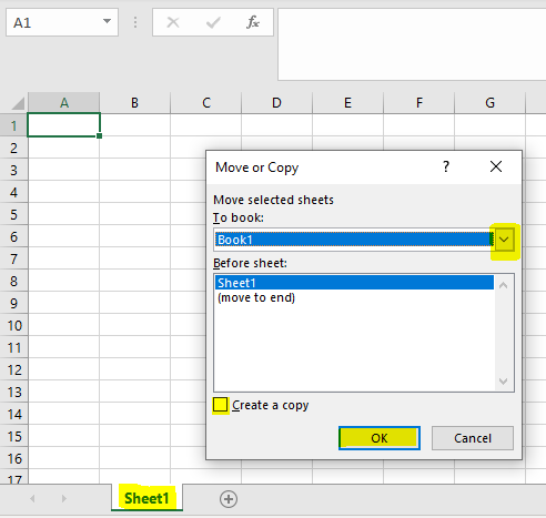
Make sure everything is saved as you want it, then open both the source workbook (the book that contains the data you want to move) and the target workbook (the book that is the destination for the data). In the source workbook, locate the worksheet you want to move or copy, then right click it and select either ‘Move’ or ‘Copy.’
In the resulting window, you’ll be able to select the destination workbook as well as specify where the worksheet should be placed. It’s best practice to click the ‘Create a copy’ checkbox to make sure all the data is copied over, then you can delete the worksheet from the source workbook if needed.
Add multiple rows or columns at once
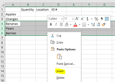
Adding rows and columns one by one can be a pain, particularly if you’re trying to insert them in the midst of existing data.
All you have to do is highlight the number of rows or columns after the row or column where you want them inserted, then right click and select ‘Insert.’ Excel understands that the number of rows/columns you selected is the number you want inserted.
Group/ungroup columns to hide detail data
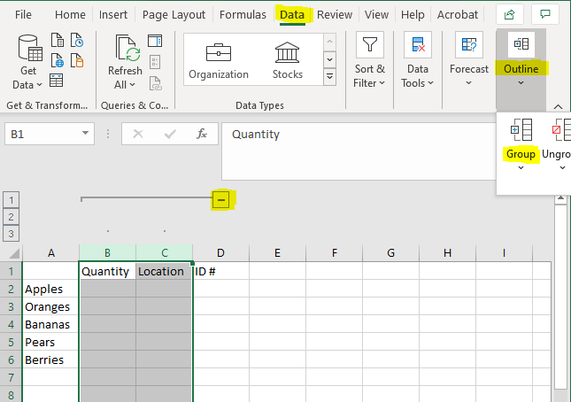
To keep things simple and easier to read, hiding data can be incredibly helpful since you sometimes need a extra data to manipulate the data you want to visualize. Grouping is a simple way to visualize only what you want and still allow the viewer to see the hidden data with a single click.
Select the columns you want grouped, then go to Data > Outline, and click ‘Group.’ A minimize/maximize icon will appear above the selected columns that you can toggle. Just be aware that this function will hide all columns selected so it’s particularly good for showing results. You can also do this with rows.
Filter data to surface what you want
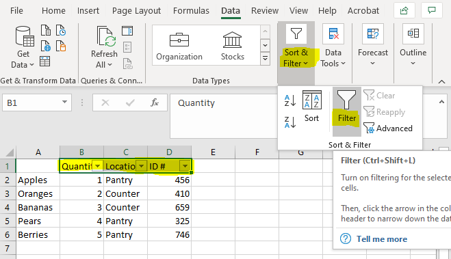
Because of the way Excel tools work, it can be much easier to start with all of the possible data that pertains to your task and then filter it down to exactly what you’re looking for instead of manually adding each little thing.
To filter your data, make sure you have column headings in place by naming each column in the first row. Then select the cells in the first row that contain your column headings and go to Sort & Filter > Filter. You’ll then see drop down arrows next to each column heading which you can then use to filter down on specific data in each column.
Copy a formula across rows or down columns
When you get your formula exactly where you want it, you can copy it down a range and Excel is smart enough to know to apply that same formula to the range of data specific to that paste destination. For instance, if you have a formula on cell A3 that adds A1 and A2, you just click on cell A3 and use the small drag box that appears in the lower right to apply that same formula to as many rows as you like. So B3 will add B1 and B2, and so on.
Continuing a series down a column or across a row
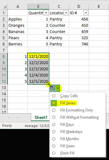
Speaking of the cell drag function, you can easily create a series using the same method. This series can be numerical, dates, and other types of data. Just put the start value (like 1 or 12/1/2020) in a cell and then click on the cell. Use the drag box that appears in the lower right to drag it in any direction you like to create a running series based on the start data.
You may need to use the menu that appears once you drag your cells to select ‘Fill series.’ You’ll also see a list of other options that can very helpful to specify the exact data you want to result in the series cells.
Transfer columns to rows or vice versa
Sometimes the layout you begin with doesn’t quite work for you. You can quickly convert rows to columns or columns to rows just by selecting the data you want to convert and copying it. Then click on the cell where you want the data to start and right click it to select ‘Paste Special.’
Click the ‘Transpose’ checkbox and ‘OK,’ then your data will appear in a converted layout.
![]()
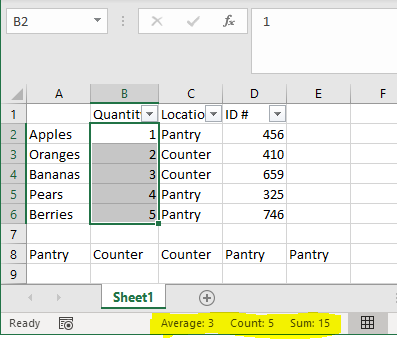
Seeing the basic stats of your data
Sometimes the simplest things seem the hardest when you’re working with tons of rows, columns, and data. If you just want to see the simple statistics of your data—like total cell count, sum of selected cells, or the average of them—just select the data you’re interested in and look at the bottom of the spreadsheet. It automatically appears for you!
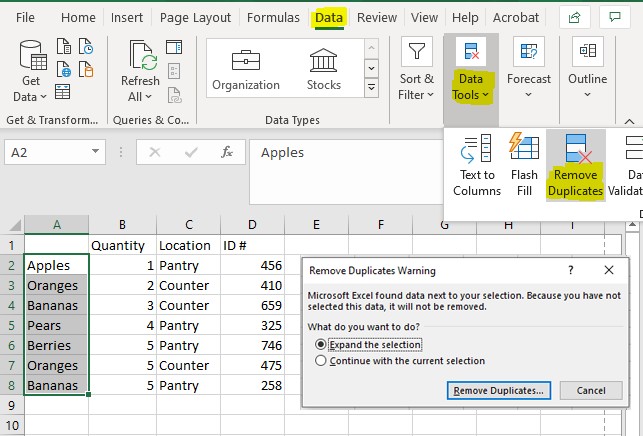
Remove duplicate data or sets of data
Larger sets of data can definitely lead to duplicates, especially when you start with all of the possible data you might need and are attempting to whittle it down to the necessary data.
To remove your duplicates, highlight the row or column that you want duplicates removed from, then go to Data > Data Tools > Remove Duplicates. The new window that pops up will allow you to remove all of the data that relates to the identified duplicates (in the case below, all of rows 7 and 8) or just remove the data that you selected.
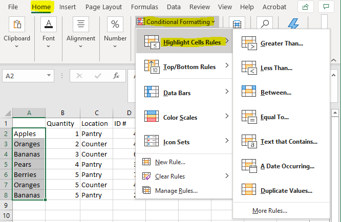
Pop out specific data with color text or highlights
If you’d like to easily pop out or flag data that exists in your worksheet, but you don’t necessarily need to change your data, you can use conditional formatting to highlight them or change the text color.
Select the group of cells where you want to find specific values (you can even select and check the whole worksheet if you like). Then go to Home > Conditional Formatting > Highlight Cell Rules. From there, you can select a variety of data identification filters such as looking for data greater than, less than, or equal to a certain value and specific dates.
More on the way
We know this is just like a drop in the ocean of how to use Excel, so we’ll have more tips and tricks coming for you in future posts. If you’re interested in more of our ‘How to’s or ‘Tips & Tricks,’ just take a look at our blog for great ideas around how to make the most of your business applications.